小程序投票/平板电视seo优化关键词

首先我们看公式：

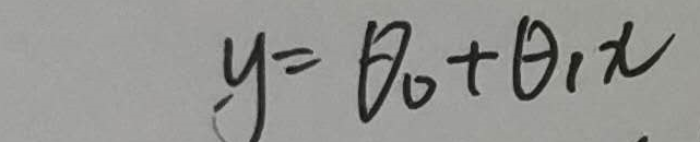
这个是要拟合的函数

然后我们求出它的损失函数， 注意：这里的n和m均为数据集的长度，写的时候忘了

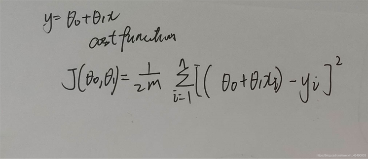
注意，前面的theta0-theta1x是实际值，后面的y是期望值

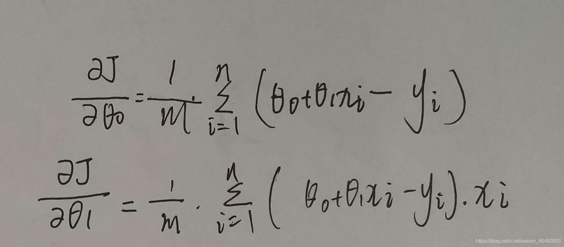
接着我们求出损失函数的偏导数：

最终，梯度下降的算法：

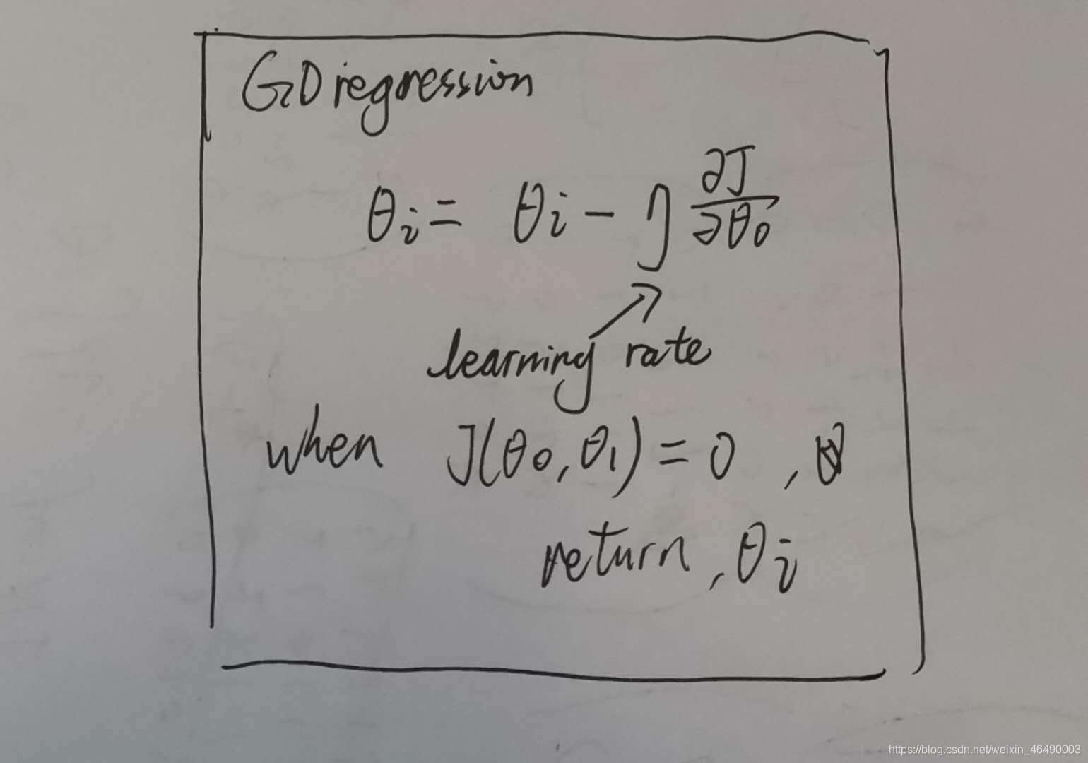
学习率一般小于1，当损失函数是0时，我们输出theta0和theta1.

接下来上代码！

class LinearRegression():

def __init__(self, data, theta0, theta1, learning_rate):

self.data = data

self.theta0 = theta0

self.theta1 = theta1

self.learning_rate = learning_rate

self.length = len(data)

# hypothesis

def h_theta(self, x):

return self.theta0 + self.theta1 * x

# cost function

def J(self):

temp = 0

for i in range(self.length):

temp += pow(self.h_theta(self.data[i][0]) - self.data[i][1], 2)

return 1 / (2 * self.m) * temp

# partial derivative

def pd_theta0_J(self):

temp = 0

for i in range(self.length):

temp += self.h_theta(self.data[i][0]) - self.data[i][1]

return 1 / self.m * temp

def pd_theta1_J(self):

temp = 0

for i in range(self.length):

temp += (self.h_theta(data[i][0]) - self.data[i][1]) * self.data[i][0]

return 1 / self.m * temp

# gradient descent

def gd(self):

min_cost = 0.00001

round = 1

max_round = 10000

while min_cost < abs(self.J()) and round <= max_round:

self.theta0 = self.theta0 - self.learning_rate * self.pd_theta0_J()

self.theta1 = self.theta1 - self.learning_rate * self.pd_theta1_J()

print('round', round, ':\t theta0=%.16f' % self.theta0, '\t theta1=%.16f' % self.theta1)

round += 1

return self.theta0, self.theta1

def main():

data = [[1, 2], [2, 5], [4, 8], [5, 9], [8, 15]] # 这里换成你想拟合的数[x, y]

# plot scatter

x = []

y = []

for i in range(len(data)):

x.append(data[i][0])

y.append(data[i][1])

plt.scatter(x, y)

# gradient descent

linear_regression = LinearRegression(data, theta0, theta1, learning_rate)

theta0, theta1 = linear_regression.gd()

# plot returned linear

x = np.arange(0, 10, 0.01)

y = theta0 + theta1 * x

plt.plot(x, y)

plt.show()

到此这篇关于python 还原梯度下降算法实现一维线性回归 的文章就介绍到这了,更多相关python 一维线性回归 内容请搜索脚本之家以前的文章或继续浏览下面的相关文章希望大家以后多多支持脚本之家！